This file type includes high resolution graphics and schematics when applicable.
Resonators with high quality factors (Qs) are used throughout high-frequency circuits. For example, matching networks are most efficient when constructed with components having high unloaded Qs. By increasing the amount of stored energy to the loss of a circuit, it is possible to improve its unloaded Q. Fortunately, a low-cost commercial computer-aided-engineering (CAE) program can help design high Q transmission-line resonators that are electrically short (less than one-quarter wavelength).
In a multisection lowpass filter, the insertion loss is inversely proportional to the average unloaded component Q (QU).1 For a single resonator, the insertion loss in dB approaches zero as the ratio of unloaded to loaded Q becomes infinitely large. For a parallel LC resonator, this implies that the individual component Q will need to be large compared to the loaded Q (terminated circuit Q) for low insertion loss.
A variety of oscillator performance parameters can benefit from a high-Q resonator, including phase noise and frequency drift (long-term frequency stability). It has been shown that the single-sideband (SSB) phase noise of a feedback oscillator is in part inversely related to the square of the loaded circuit Q.2 Other factors, such as amplifier noise factor and signal power, affect overall phase noise in direct proportion only to their magnitudes. The exponential (second power) influence of the Q factor gives it a prominent impact on oscillator phase noise.
A circuit's Q can basically be defined as equal to two times the product of π and the ratio of the maximum energy stored to the energy dissipated per cycle. In an electrical circuit, energy is stored in the electric or magnetic fields associated with reactive circuit components and electrical energy is lost (to heat) whenever current flows through a resistance. From this basic definition, the way to improve Q is to increase the ratio of stored energy to losses in a circuit. Although how to achieve this may not always be apparent, a commercial software program that combines synthesis with simulation, the LINC2 program from Applied Computational Sciences (Escondido, CA), can simplify the task.
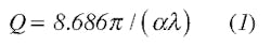
A section of transmission line shorted at one end will form a resonant circuit at the frequency represented by its quarter wavelength (90-deg. electrical length). Ports coupled into and out of the top side of the resonator form a bandpass circuit similar to a parallel-resonant resistive-inductive-capacitive (RLC) circuit. The Q of this full-length (quarter-wave) resonator can be found from:
where:
α = the line loss (dB/in.), and
λ = the wavelength (in.).
As an example, consider a resonator constructed on FR-4 printed-circuit-board (PCB) material with the following material properties at 1 GHz: relative dielectric constant, εr = 4.6, dielectric height = 30 mil, 50-Ω trace width of 54.4 mil on 0.5-oz. copper, α = 0.094 dB/in., and λ = 6.35 in. Using these values in Eq. 1 gives Q = 27.3/0.094/6.35 = 45.7. Because of the lossy PCB material this is not a very high-Q resonator, and higher Q values could be achieved by using lumped elements. The Q of a parallel LC resonator is largely determined by the Q of the inductor, which can be as high as 60 or more at this frequency for a surface-mount 0603 size part. However, by shortening the microstrip resonator and restoring resonance with a low-loss shunt capacitor, the Q can be increased by 50 to 100 percent. The Q for the printed resonator can exceed that of the lumped LC version without the expense of the discrete inductor.
The unloaded Q of a nonresonant shorted section of transmission line can be determined as a function of its length by the relation3:
where:
ω = 2πf
and the real and imaginary components of the line impedance are:
R = Z0sinh(2αl)/
X = Z0sin(2βl)/
where:
α is the attenuation factor, and
β = 2π/λ, the propagation constant of the line.
Figure 1 shows the Q as a function of length (to one-quarter wavelength) for transmission-line sections with varying amounts of loss.
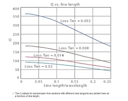
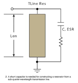
The bottom curve plots the Q for a 50-Ω trace on 30-mil-thick FR-4 PCB with dielectric loss tangent of 0.02. The top trace shows what can be achieved with low-loss PCB material having one-tenth of this loss tangent (or 0.002). Constructing a resonator from the sub-quarter-wavelength line requires a shunt capacitor to restore resonance as shown in Fig. 2.
The capacitor has loss that will add to the total losses of the resonator and thus lower the Q. Figure 1 represents the unloaded Q of the line by itself, which would be equal to the Q of a resonator in the limiting case of an ideal (lossless) capacitor and transmission-line combination.
Figure 3 plots the unloaded Q of the resonator in Fig. 2 for various values of effective series resistance (ESR) for a capacitor resonating with the section of transmission line shown in Fig. 1 (with loss tangent of 0.008).
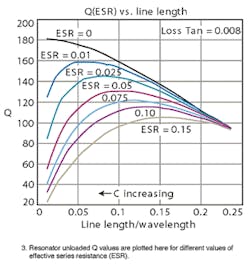
For an ideal capacitor with ESR = 0 (top trace of Fig. 3), the resonator Q is the same as the transmission line Q in Fig. 1. Note that as the line length decreases the value of the capacitor increases to maintain resonance at the desired frequency (1 GHz in this case). As the resonator length is shortened (C increasing), the Q rises above the quarter-wavelength value of Q = 8.686π/(αλ). However, for all resonating capacitors with ESR values greater than zero, the Q eventually falls again.
Page Title
Figure 4 helps to show the effect of capacitor ESR on capacitor Q (and ultimately resonator Q).
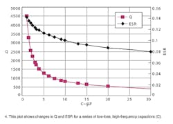
It plots the Q and ESR for a series of low-loss, high-frequency capacitors, with the Q of the capacitor equal to 1/, where C is capacitance. For a given frequency and constant ESR, the capacitor's Q would decrease inversely with C. Although this is not quite the case, the ESR decreases slowly enough with increasing C values that the effect is the same. Starting at a capacitance of 1 pF and a Q of several thousand (for data taken at 200 MHz), the Q drops rapidly with increasing capacitance.
Since the overall Q of the resonator in Fig. 2 is Qresonator = 1/c) +(1/Qt)>, Fig. 4 explains the eventual decline in the resonator Q for very short line lengths and large capacitor values. The falling capacitor Q (Qc) finally overtakes the increasing transmission-line Q (Qt). However, before it does, there is an optimum line length where maximum resonator Q is achieved.
Equation 2 does a fair job of predicting the transmission line Q up to the vicinity of self-resonance at one-quarter wavelength. However, as the resonator length exceeds 90 percent of a quarter wavelength, Eq. 2 begins to lose accuracy. Fortunately, the LINC2 program uses a proprietary algorithm to accurately calculate the Q of a parallel transmission-line/capacitor resonator through all ranges of line length up to and including one-quarter wavelength. In performing the calculations, LINC2 automatically takes into account the PCB material and the type of transmission-line (microstrip or stripline) structure (Fig. 5).
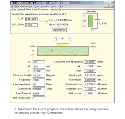
In using this program, the first step in the design process requires entering information about the PCB material and the metal (trace) parameters. From this information, the physical dimensions of the metal strip are calculated and displayed. In addition, the software computes other physical properties, including the line loss and unloaded resonator Q for any given type of capacitor. Upon entering the capacitance and ESR for the resonator capacitor, the strip length and Q of the resonator are displayed.
An important feature of the program is its ability to optimize the resonator Q by finding the optimum capacitor value and line length for maximum Q. Since all calculations are based on the specified metal and substrate material, different PCB materials can be quickly analyzed for their ability to support a resonator design for a desired Q factor.
A design example will involve determining the unloaded Q for a full-length (quarter-wavelength) resonator on 50-Ω microstrip using the PCB material of Fig. 5, as well as the maximum unloaded Q for a (shorter) 50-Ω microstrip resonator on the same PCB material. The line length and the value of a resonating capacitor (one capacitor with ESR of 0.025) must also be calculated for that maximum Q value. In addition, it will be necessary to compute the percent improvement in Q for the shorter resonator compared to the full-length resonator. Finally, the design example will involve verifying the Q of the shorter resonator through a computer simulation.
To complete this design example with the LINC2 program, the Q for a quarter-wavelength resonator can be obtained by entering a very small value for C (such as 0.001 pF). This effectively removes the loading capacitor and lets the resonator go to full length. After entering the material specifications (from Fig. 5) and 0.001 for the value of C, the program reports an unloaded Q of 92. The Q can also be calculated manually from Eq. 1. Substituting the appropriate values yields Qu = 27.3/1.867/0.161 = 91, which is close to the program-computed value.
Entering 0.025 for the capacitor's ESR and clicking the "Optimize Q" button in LINC2 yields a Qu,max of 146.93, a line length of 13.536 mm (note that the resonator strip has been shortened to 30.225 deg.), and C of 5.46 pF (see Fig. 5). The quarter-wavelength resonator has a Q = 92 while the short resonator produced a Q = 146.93. The percentage improvement in Q is 100(146.93 − 92)/92 = 59.7 percent. Figure 5 includes all of the information needed to physically construct the shorter, high-Q resonator. The microstrip resonator, capacitor (with ESR modeling resistor), and PCB material specification can be placed in a LINC2 schematic window and simulated.
Figure 6 shows the LINC2 schematic for the short resonator with the circuit connected to input and output measurement ports.

High-impedance (5000 Ω) measurement ports were used to lightly load the resonator, allowing for enough insertion loss to aid the calculation of unloaded Q as a function of loaded Q and insertion loss (Eq. 3).
From the simulation, the unloaded Q (Qu) can be calculated from the simulated loaded Q (Ql) by:
where:
IL_dB = the insertion loss (in dB) at the center frequency, Fc, and
Ql = Fc/(BW_3dB).
Figure 7 offers simulation results for the short resonator, with markers placed at the upper and lower 3-dB points.
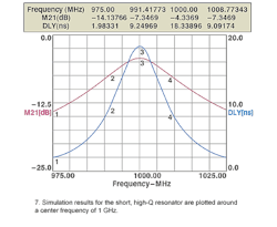
The plot indicates a 3-dB bandwidth (BW_3dB) of 1008.77343 − 991.41773 = 17.3557. The insertion loss (IL_dB) is 4.3369 dB.
The simulated loaded Q is:
Ql = Fc/(BW_3dB) = 1000/17.3557 = 57.62.
The unloaded Q (Qu of the resonator can now be obtained from Eq. 3 as:
Qu = 57.62 / = 146.6.
This agrees very closely with the unloaded Q reported by the synthesis program (Qu = 146.9 in Fig. 5). This verifies (through simulation) the design and physical construction details proposed by synthesis.
The loaded Q can also be calculated from the group delay according to the relation:
Ql = ωTd/2
where:
ω = 2πf and
Td = the time delay.
Equation 3can now be rewritten as:
The delay reported in the simulation results (Fig. 7) is 18.34 ns. Therefore, the resonator's unloaded Q by this calculation is Qu = (3.142 × 1 × 18.34)(2.544) = 57.62 × 2.544 = 146.6, which is the same result obtained in the calculation based on the bandwidth.
Page Title
Figure 3 indicates that the resonator Q cannot be improved appreciably above the quarter-wavelength value unless a very low-loss capacitor is used. In the example above, the ESR of the capacitor was 0.025 Ω. If a single capacitor with that value of ESR is not practical, multiple capacitors can be placed in parallel with the resonator strip to obtain the necessary value. For example, four 1.3-pF capacitors all with ESR of 0.1 Ω combine in parallel to obtain the approximate 5-pF capacitance and 0.025 Ω ESR used in the example. Measurements taken in the lab with a commercial vector network analyzer verify the improvement in Q for a resonator constructed with multiple parallel capacitors.
While shortening a resonator's length also improves its Q, the smaller size is also a desirable result. In this design example, a full-length (90-deg.) resonator would be 1.5 in. long at 1000 MHz, a length that may be impractical for a miniature voltage-controlled-oscillator (VCO) PCB. The shorter resonator, with length of only 0.5 in., is much more suited to the design of more compact, modern VCOs.
In summary, LINC2 is a high-performance RF and microwave circuit design and simulation program with many value-added features for automating design tasks, including circuit synthesis. This example showed how LINC2 can quickly and easily design high-quality-factor resonators to meet a given Q requirement and evaluate the suitability of different PCB material in meeting those objectives. More information about LINC2 and Applied Computational Sciences can be found on the website at www.appliedmicrowave.com.
REFERENCES
- T. Koryu Ishii, Handbook of Microwave Technology, Academic Press, New York, 1995, pp. 185-186.
- D.B. Leeson, "A Simple Method of Feedback Oscillator Noise Spectrum," Proceedings of the IEEE, February 1966, pp. 329-330.
- Peter Vizmuller, RF Design Guide, Artech House, Norwood, MA, 1995, p. 235.
This file type includes high resolution graphics and schematics when applicable.
