This file type includes high resolution graphics and schematics when applicable.
Coaxial cables are essential to many RF/microwave applications, being the external transmission lines that connect high-frequency signals from one point to another. Unfortunately, whether used in a circuit, a system, or in a test setup, coaxial cables can develop unseen faults that may be anywhere in their length. Finding those faults can often be challenging, typically requiring the use of time-domain reflectometry (TDR) which operates much like a radar system; it sends a signal with fast edge into the cable and measuring the time required for the reflected signal edge to return from the fault.
Analysis of the reflected signal gives insight into the location and type of fault. The resolution of a distance measurement depends on the risetime of the pulsed test signal, which must be in the picosecond range to resolve a cable fault that may be only inches away from the test signal connection. In addition, the accuracy of TDR measurements will suffer when working with transmission lines which cannot support these high frequencies; attenuation is increased as the distance to fault increases.
Fortunately, there is an alternative approach to finding faults in coaxial cables, by means of a new frequency-domain fault detection (FD)2 method.
Cable fault detection based on TDR techniques is accurate and reliable, although the measurements can be complex and require sophisticated and often expensive test equipment, such as a high-frequency oscilloscope and pulse generator or a single integrated TDR tester. The (FD)2 method does not require specialized test equipment or very high test frequencies to determine the location of a cable fault.
In fact, with the (FD)2 approach, the longer the distance to the fault, the lower the frequency required to find it. The test method was easily capable of resolving the addition of a 0.8-in.-long BNC adapter to the end of a 2-ft.-long coaxial cable. It should be noted, however, that while a TDR measurement determines both the location and nature of a cable fault (open, short, or complex impedance), the (FD)2 approach only provides the location of a simple fault (an open or short). In many cases, this is all that is needed.
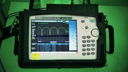
For the measurement examples presented in this report, a model MS2720T Spectrum Master spectrum analyzer with integrated tracking generator from Anritsu Co. was used. The base model in this series of instruments operates from 9 kHz to 9 GHz with resolution bandwidths from 1 Hz to 10 MHz. For the purpose of performing (FD)2 cable fault detection, however, this is quite a suitable frequency range performance in a relatively small, battery-powered package. In fact, to perform (FD)2 cable fault detection, all that is required is a calibrated frequency source (such as a synthesized frequency generator or frequency generator with a frequency counter) and a means of detecting its relative amplitude (such as an oscilloscope or RF power meter).
Principle of Operation
Like fault detection using TDR, the (FD)2 method sends a signal down a cable and measures the reflected versions of that original signal. However, the (FD)2 approach uses a continuous sinewave signal rather than the high-speed pulsed signals of TDR measurements. Like TDR measurements, signal reflections will occur at a cable fault due to the interruption in the transmission line impedance at that point, and the reflected signals will travel back towards the signal source.
At particular frequencies and line lengths, the reflected signal wave will be completely out of phase with the initial forward-wave signal, resulting in cancellation of the signal wave. By measuring the frequencies at which these cancellations (or nulls) in the signal waves occur, it is possible to determine the distance from the signal source to the cable fault.
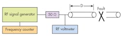
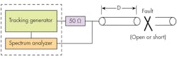
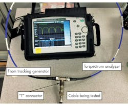
The measurement setup for the (FD)2 method is very similar to that used for TDR measurements, except that the pulse generator is replaced by a signal generator and the oscilloscope is replaced by an RF voltmeter (Fig. 1). When a spectrum analyzer with an integral tracking generator is used, the test setup simplifies to the configuration shown in Fig. 2. A photograph of the actual measurement setup used for the examples in this article is shown in Fig. 3.
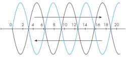
As noted, the returning signal waves reflected from the fault will result in cancellations with the forward wave when the two waves are out of phase with each other; a null will occur whenever the reflected wave is delayed by 180 deg. (or ½ wavelength) and repeated every 360 deg. that the wave travels (Fig. 4). These nulls occur according to the relationship in Eq. 1:
2d = λ/2, 3λ/2, 5λ/2, (2n + 1) λ/2, …
with n = 3, 4, 5, . . . (1)
where d is the distance to the fault and λ is the wavelength of the cable at a frequency of interest.
Similarly, peaks occur when the reflected wave is in phase with the forward wave, and delayed by an integral number of wavelengths, as shown in Eq. 2:
2d = λ, 2λ, 3λ, nλ, …
with n = 4, 5, 6, . . . (2)
Substituting λ = v/f, where v is the velocity of propagation of the cable (approximately 0.6c or three-fifths the speed of light) and f is the test frequency, and performing some algebraic manipulation, it is possible to find that nulls and peaks will occur in an open-circuited cable for the conditions shown in Eqs. 3a and b:
Nulls occur at
f = (1/4)(v/d), (3/4)(v/d), 5/4)(v/d), [(2n +1)/4](v/d), . . . with n = 3, 4, . . . (3a)
Peaks occur at
f = (1/2)(v/d), (2/2)(v/d), 3/2)(v/d), (n /2)(v/d), with n = 4, 5, 6, . . . (3b)
The difference in frequency between two successive nulls or peaks can be found by Eq. 4:
Δf = (1/2)(v/d) (4)
or by solving for the distance to the fault in the cable, d, by means of Eq. 5:
d = (1/2)(v/Δf) (5)
By knowing the values of v and Δf, it is possible to find the value of d.
A similar analysis can be performed for a shorted cable, where Eqs. 4 and 5 still apply, although it should be noted that the (FD)2 method cannot differentiate between open-circuit and short-circuit cable faults.
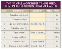
Prior to performing cable fault detection with the (FD)2 method, it is necessary to calibrate cable velocity, v, for the particular cable using a known length of the same kind of cable as the transmission line that is being tested. For this purpose, Eq. 4 is solved for v as shown in Eq. 6:
v = (2d)(Δf) (6)
Finding the distance to the fault is then simply a matter of measuring the frequency difference between successive nulls and applying Eq. 5. Although either peaks or nulls could be measured for this purpose, it is easier to measure nulls because they are sharper.
Explore an Example
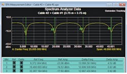
To demonstrate an example of using this fault-finding technique, first calibrate the test system using a known length of cable of the same type to be tested. Simulate a break in the known cable length and then find the distance to the fault. Calibration can be performed by connecting an unterminated 7.5-m length of cable to the test system (two 3.75-m-long cables coupled together). Equation 6 can be applied with an added 3-in. length for the arm of the T-connector in the test setup of Fig. 3 to find (as shown in Fig. 5):
v = 2(3.75 m + 3 in.)12.9974 MHz
v = 1.969 × 10⁸ m/s
The fault in the cable can be simulated by breaking the coupling between the two 3.75-m cables, so that the correction answer, 3.75 m, is already known.
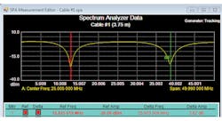
Using Eq. 5 and then subtracting out the 3-in. length of the T-connector in the test setup (Fig. 3), it is possible to calculate the additional cable length (as shown in Fig. 6):
d = (1/2)[(1.969 × 108 m/s)/(25.904 MHz)] – 3 in.
d = 3.725 m
An error of 25 mm (about 0.67%) from the actual known 3.75-m distance is due in large part to the (lack of) frequency resolution of the spectrum analyzer. Higher analyzer resolution can be achieved by reducing the frequency span so that just a single null is shown on the analyzer’s display screen.
In short, the (FD)2 method provides a simple means to find the distance to a gross fault, such as an open or short, in a transmission line using only a relatively low-frequency signal generator and some form of amplitude measuring instrument, such as a general-purpose spectrum analyzer. The new method eliminates the need for complex TDR techniques and more expensive test equipment for finding faults in coaxial cables.
Herb Perten, Chief Scientist
Electro-Miniatures Corp., 68 W. Commercial Ave., Moonachie, NJ 07074; (201) 460-0510
Looking for parts? Go to SourceESB.
This file type includes high resolution graphics and schematics when applicable.
