Testing The Limits Of IEEE 802.11ac

This file type includes high resolution graphics and schematics.
As the IEEE 802.11ac wireless standard evolves, it continues to breed new challenges for those tasked with testing and measuring these wireless systems. With products based on the IEEE 802.11ac standard continuing to add higher density modulation schemes, wider bandwidths, and more multiple-input, multiple-output (MIMO) antenna configurations, testing these products calls for higher-performance test instruments and measurement strategies.
Related Articles
• Getting A Grip On IEEE 802.11ad
• What’s The Difference Between IEEE 802.11ac And 802.11ad?
• Take An In-Depth Look At IEEE 802.11ac
Starting with their release in 1997, the IEEE 802.11 family of wireless communications standards has evolved to deliver higher data rates: from 2 Mb/s in 1997 to nearly 7 Gb/s at present. In 2012, various IEEE 802.11 amendments were consolidated into a single standard that includes direct-sequence-spread-spectrum (DSSS, IEEE 802.11b), orthogonal-frequency-division-multiplexing (OFDM, IEEE 802.11a/g), and high-throughput (HT, IEEE 802.11n) specifications. This paved the way for the imminent release of the very-high-throughput (VHT) IEEE 802.11ac specification. While the HT specification improved the maximum throughput by an order of magnitude over the previous OFDM specification, the VHT (IEEE 802.11ac) specification boosts the maximum throughput by another order of magnitude. As Table 1 shows, the VHT specification builds on technologies developed for previous IEEE 802.11 substandards.
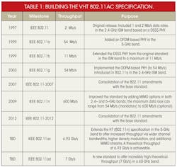
An important result of the IEEE 802.11-2012 amendment was the change in nomenclature from previous amendments. While the wireless industry has long referred to Wi-Fi technologies by their amendment letter (such as IEEE 802.11a or IEEE 802.1g), these technologies were renamed and referred to as DSSS, OFDM, etc. Since 1997, each new amendment to the 802.11 standard has attempted to increase data throughput compared to previous generations. As was seen with HT, increases in data rate have been accomplished through a variety of mechanisms. These include more spatial streams through the use of MIMO, wider channel bandwidths (and hence more data subcarriers), and even higher code rates. Equation 1 shows show to perform a quick calculation of the data rates of OFDM-based signals:
Data rate = Spatial streams x data carriers x symbol rate x bits per symbol x coding rate x duty cycle (1)
As noted, the VHT specification produces a maximum data rate roughly an order of magnitude higher than HT and two orders of magnitude higher than OFDM. In fact, the improvements in data rate can be easily understood by comparing key parameters for the specifications (Table 2). For variable parameters, Table 2 lists those yielding maximum throughput. The 160-MHz and 80 + 80-MHz options for VHT share the same number of subcarriers/pilots.
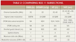
As Table 2 shows, the VHT specification allows for channel bandwidths as wide as 160 MHz, or four times greater than the 40-MHz maximum bandwidth offered by HT (or alternately, eight times greater than the 20-MHz bandwidth provided by OFDM). Wider bandwidths allow a greater number of data subcarriers to be handled. Moreover, the VHT specification uses a slightly higher concentration of data carriers per channel bandwidth versus the HT and OFDM specifications. For example, 91.4% (468/512) of the subcarriers in a 160-MHz VHT channel are data subcarriers, versus 75% (48/64) for OFDM.
Table 2 also shows that the increase in spatial streams from OFDM through VHT produces one of the largest contributions to maximum data rate. The increase in spatial streams through the use of MIMO technology increased by a factor of four from the OFDM specification using single-input, single-output (SISO) antenna techniques to the HT specification with 4 x 4 multiple-input, multiple-output (4 x 4 MIMO) antenna methods. Moreover, the VHT doubles the number of spatial streams again, going from 4 to 8.
This file type includes high resolution graphics and schematics.
Increased Complexity
This file type includes high resolution graphics and schematics.
Finally, the last big improvement, moving from OFDM to HT to VHT, is the increase in modulation/coding scheme complexity. For example, the HT specification introduced the 5/6 coding rate when using a 64QAM modulation scheme, resulting in an 11% increase in data rate over the 3/4 coding rate of OFDM, all other things being equal. The VHT specification also introduced the 256QAM modulation scheme, resulting in a 33% increase in the number of bits per symbol due to the higher order modulation employed. The 64QAM format has 6 b/symbol [log2(64)] while 256QAM pushes this to 8 b/symbol [log2(256)].
However, the dramatic improvement in throughput in the VHT specification comes at the expense of higher performance requirements and the needs for more complex test equipment. For example, the modulation accuracy required for devices to use more complex schemes such as 256QAM requires RF test systems to have greater linearity and better phase noise performance than what was required for previous iterations of the standard. More specifically, key transmitter measurements—such as error vector magnitude (EVM)—require careful attention to various settings on the RF signal analyzer used to measure the transmitter.
Measuring the modulation accuracy of a transmitter is one of the most important metrics in ensuring its intended performance. The key figure of merit usually considered, with respect to modulation accuracy, is EVM. To understand an EVM measurement, it is first necessary to realize that signals can be represented in the Cartesian domain as polar coordinates (Fig. 1). Each transmitted “state” of the carrier is called a “symbol” and is used to communicate a unique digital bit stream. For modulation schemes such as the 16QAM scheme shown in Fig. 1, each symbol is assigned a unique bit stream of four unique logical bits. To transmit a digital message bitstream, the message is divided into groups of 4 b, and the transmitter generates one symbol at a time at the prescribed “symbol rate.” At the other end, a receiver decodes each symbol and—applying the appropriate symbol mapping—reconstructs the original bit stream.
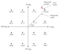
1. This is a constellation diagram representing 16QAM modulation.
As modulation schemes increase in complexity (i.e., from 16QAM to 256QAM), the relative phase and magnitude difference between adjacent symbols gets smaller. The EVM measurement is the primary metric of modulation quality, and is defined as the ratio of an “error vector” with the “magnitude vector.” The error vector can be graphically described as the difference in magnitude between a symbol’s measured phase and magnitude and its ideal location. The magnitude of this vector difference is known as the EVM. In order to measure EVM, a vector signal analyzer (VSA) which can measure both the amplitude and phase of received signals is required.
In practical use, accurately measuring the transmit EVM of an IEEE 802.11ac device requires paying careful attention to the signal-to-noise ratio (SNR) of the RF signal analyzer. The IEEE 802.11ac specification requires a transmitter to have a transmit EVM performance of -32 dB, inherently requiring that test instruments can measure EVM that is as much as 10 dB better (-42 dB). Moreover, the high peak-to-average power ratio (PAPR) of OFDM signals (often to 13 dB) used in IEEE 802.11ac requires that a signal analyzer have a SNR of upwards of 60 dB. As a result, characterizing the transmitter requires maximizing the SNR of the signal analyzer.
Appropriately setting the reference level of a signal analyzer is one of the easiest ways to maximize the SNR of the measuring instrument. Many instruments will offer an auto-level setting that will dynamically determine the peak amplitude of the IEEE 802.11 signals and set the reference level accordingly. However, using this option comes at the expense of measurement time when automating measurements. With the inherently greater measurement times of VHT signals (owing to the denser modulation options), it is desirable to set the reference level manually, thus reclaiming the time lost in this automation.
To maximize EVM performance, understanding the PAPR of the signal itself is a useful start to setting the reference level. Most OFDM signals have a PAPR that can range from 10 to 12 dB. In addition, most RF signal analyzers are designed so that their maximum clipping level occurs 6 to 8 dB above the reference level. As a result, the ideal setting for the reference level of a typical signal analyzer is usually 4 to 8 dB above the average power of the signal. Setting the reference level too low will result in the captured signal clipping and will degrade the measured EVM. If the reference level is set too high, the noise floor of the signal analyzer would influence the measurement result—also degrading the EVM measurement.
To illustrate this point, a model PXIe-5644R vector signal transceiver (VST) from National Instruments was used to generate and analyze an IEEE 802.11ac signal and various modulation-and-coding-scheme (MCS) rates and channel bandwidths. The PXIe-5644R is a signal generator and an analyzer in compact PXI module format. It covers 65 MHz to 6 GHz with an 80-MHz instantaneous bandwidth and features an impressive noise floor of -161 dBm/Hz . The output of the transceiver’s signal generator was directly connected to the input of the onboard signal analyzer. With the signal generator producing the IEEE 802.11ac signal at a constant power level, a series of modulation accuracy measurements were made while varying the reference level (Fig. 2).
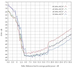
2. Error vector magnitude (EVM) is shown as a function of reference level.
The x-axis is the difference between the reference level and the average packet power, in dB. The 0-dB mark represents the reference level and is equal to the average packet power. Negative numbers correspond to the reference level being set below this average power level, while positive values are a reference level set higher than the average power level.
The EVM measurement is dramatically degraded when the reference level is set too low, as clipping inside the signal analyzer significantly affects modulation quality. Moreover, as the reference level is slowly increased, the noise floor of the signal analyzer itself increasingly becomes the largest contributor to measurement uncertainty. The optimal reference level for this particular signal is to about 6 dB higher than the average power as the signal (Fig. 2).
This file type includes high resolution graphics and schematics.
Reference Rule Of Thumb
This file type includes high resolution graphics and schematics.
The results of this experiment yield a rough rule of thumb for setting the reference level. The PAPR of the OFDM signals detailed earlier was extracted (Fig. 3) from the complementary cumulative distribution function (CCDF). It might make sense that the optimum reference level would be set at the sum of the expected average packet power and the PAPR, as this is the maximum expected signal level.
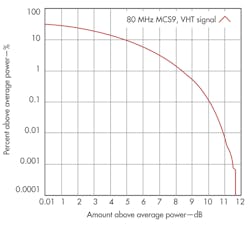
3. This plot shows the complementary cumulative distribution function (CCDF) of an 80-MHz-bandwidth, MCS9 VHT signal.
But looking again at Figs. 2 and 3, this is not the case. While the PAPR indeed captures the ratio of the maximum power, as seen in the CCDF, the vast majority of the information is contained in a much lower power level envelope. Setting the reference level at the maximum power level instead takes dynamic range away from the majority of the packets. From the CCDF, it can be seen that the PAPR is around 11 dB. To make good EVM measurements, the reference level should instead be optimized at a delta value closer to 7 dB, or about 4 dB below the sum of the expected average and the PAPR.
Related Articles
• Getting A Grip On IEEE 802.11ad
• What’s The Difference Between IEEE 802.11ac And 802.11ad?
• Take An In-Depth Look At IEEE 802.11ac
In addition to the more stringent SNR requirements for IEEE 802.11ac signals, the larger bandwidths and more complex modulation schemes also require more signal processing to be performed during demodulation measurements. As a result, measurement times for IEEE 802.11ac signals increase over previous revisions of the standard. With measurement test times inherently increasing, it is desirable to intelligently optimize the measurement parameters with respect to measurement quality and duration.
One such parameter in making good modulation accuracy measurements is the number of averages upon which the EVM measurement is based. While IEEE 802.11 standards specify 10 averages for a measurement, this number of overages can result in significantly longer measurement times. Thus, when testing a device, the trick is to identify the number of averages required to gain the desired measurement repeatability. As Fig. 4 shows, measurement repeatability gradually improves as more averages are used to compute the measurement result.
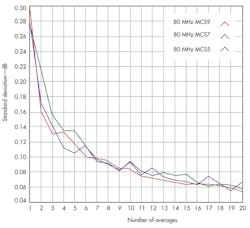
4. These traces show standard deviations of for measured EVM performance levels.
In practical use, measurement repeatability in the range of 0.1 dB is sufficient for most automated test applications. Should a wider variance be acceptable, three averages should yield good results while requiring less test time. Conversely, if repeatability is critical, increasing the number of averages will yield more consistent results at the expense of longer measurement times. When comparing measurement results, both EVM as well as test time, between different applications, it is important to also note the number of averages used in each.
In summary, the latest iteration in IEEE 802.11 specification, the IEEE 802.11ac amendment, continues to push performance forward as it adds an order of magnitude of potential throughput. Adding additional spatial streams and higher order modulation over wider channel bandwidths can be seen to be responsible for much of this greater throughput. And, as with the specification, test and measurement systems similarly require incremental improvements in items such as real-time bandwidth, improved linearity, and greater dynamic range. Optimizing available parameters in the measurements serves to maximize the capabilities of the instrumentation as well as the reliability of the results.
This file type includes high resolution graphics and schematics.
