Algorithms to Antenna: Understanding Subarray Tradeoffs in Large Antenna Arrays
In my last blog, I showed how a large array can be modeled using a 64-element phased array that operates at 66 GHz. To start, I used a cosine pattern to model each element in the antenna array. It took only a few minutes to set this up and with the model in place, I can explore beam patterns across different frequencies and beamsteering locations. I then replaced the ideal antenna element model with a microstrip patch that I designed with a few clicks of my mouse using the Antenna Designer app. The resulting antenna element design provides a higher-fidelity model.
Now, I want to relate the topic of array design back to our discussion in blog 3 on hybrid beamforming. Recall that with hybrid beamforming, you trade off cost versus performance by partitioning your beamforming architecture between the RF and digital domains.
This brings us to the topic of subarrays, where multiple antenna elements are mapped to specific RF channels. Subarrays are integrated to build up a full antenna array. Sometimes element feeds are shared across subarrays to create virtual arrays. The key point is that the total number of transmit/receive modules is less than the number of antenna elements for each subarray, which results in less required hardware in large systems.
Having less hardware is an advantage from the cost and power perspectives, but without an all-digital beamforming design, some flexibility in terms of steering resolution is sacrificed in the RF portion of the beam steering. This occurs when the same RF phase shift value is applied to each channel of a subarray. It contrasts with the all-digital case, where phase and amplitude weighting can be unique values for each channel.
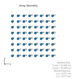
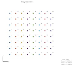
1. Shown is a 64-element uniform rectangular array without (top) and with (bottom) eight subarrays.
The next step is to evaluate these tradeoffs to obtain the best hybrid beamforming architecture for a given system. To start, you can design the antenna array as a system of subarrays. The 64-element array can be modeled with individual elements as an all-digital system (as shown in blog 4), or as an integrated set of subarrays. Figure 1 shows both array types. On the right side of Figure 1, the antenna array is built up from eight 8×1 linear subarrays, but this configuration is flexible and can be easily tailored.
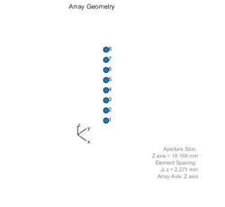
2. This figure illustrates the element pattern for patch microstrip (top) along with the 8×1 element subarray (bottom).
There are several options to move forward that illustrate how steering changes with a partitioned system. For the first case, pattern superposition is applied to generate the 3D pattern using an isolated patch element. Figure 2 shows the 3D pattern for the patch element obtained using a method of moments (MoM) solver and the corresponding subarray, which is set up as an 8×1 uniform linear array (ULA).
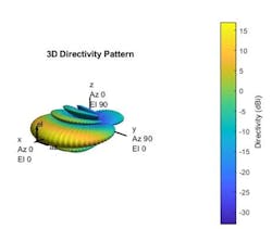
Figure 3 shows that pattern superposition generates a 3D pattern for the 8×1 subarray. As expected, the resulting beam pattern covers a broad azimuth coverage.
3. Shown is the pattern for a single 8×1 subarray.
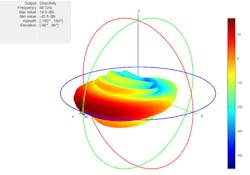
We can model a similar subarray, but rather than use superposition, we model the entire subarray with the solver to achieve higher fidelity. In Figure 4, we see the resulting array structure along with the 3D pattern.
4. In this figure, the structure (top) and pattern (bottom) for a single 8×1 ULA is shown.
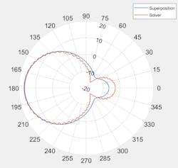
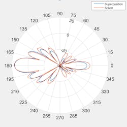
To visualize the difference between the two techniques, we compare the azimuth and elevation 2D cuts (Fig. 5).
The different techniques shown above should help you understand how model fidelity can change the predicted array performance. By extending this workflow, these types of models can be iterated to find the right subarray architecture. This is done by using the resulting subarray architecture to generate the full array design; the resulting patterns for the full array can then be evaluated across design options.
5. Shown is a comparison of subarrays modeled with superposition and full solver in azimuth (top) and elevation (bottom).
Once the partitioning is complete, the workflow can shift to maximizing the spectral efficiency to improve channel capacity. This requires that each RF chain be used to send an independent data stream. Assuming the channel is known, the unconstrained optimal precoding weights can be obtained by diagonalizing the channel matrix and extracting the dominant modes. I will discuss this topic more in a future blog.
In the next blog, I will go into more detail on modeling mutual coupling between elements in large antenna arrays.
Learn more about hybrid beamforming or email me at [email protected] with feedback or thoughts along the way.
Learn more about topics covered in this blog post:
- Phased Array Gallery (Example): This example shows how to model and visualize a variety of antenna array geometries with Phased Array System Toolbox.
- Subarrays in Phased Array Antennas (Example): This example shows how to model subarrays, commonly used in modern phased array systems, and perform analyses using Phased Array System Toolbox.
- Antenna Array Analysis (Example): This example shows how to create and analyze antenna arrays in Antenna Toolbox, with emphasis on concepts such as beam scanning, sidelobe level, mutual coupling, element patterns, and grating lobes.
- Design of Cutting-Edge Antennas and Antenna Arrays with MATLAB (webinar, 36:12): This webinar shows how MATLAB and Antenna Toolbox can help you design antennas and antenna arrays, rapidly try different configurations, and integrate them earlier at the system level.
Click here to see additional 5G, radar, and EW resources, including those referenced in previous blog posts.
About the Author
Rick Gentile
Product Manager, Phased Array System Toolbox and Signal Processing Toolbox
Rick Gentile is the product manager for Phased Array System Toolbox and Signal Processing Toolbox at MathWorks. Prior to joining MathWorks, Rick was a radar systems engineer at MITRE and MIT Lincoln Laboratory, where he worked on the development of several large radar systems. Rick also was a DSP applications engineer at Analog Devices, where he led embedded processor and system level architecture definitions for high performance signal processing systems used in a wide range of applications.
He received a BS in electrical and computer engineering from the University of Massachusetts, Amherst, and an MS in electrical and computer engineering from Northeastern University, where his focus areas of study included microwave engineering, communications, and signal processing.
