Algorithms to Antenna: Radar Target Modeling
At the International Microwave Conference 2019, we hosted a workshop that explored how to model objects in the field of view of a radar. In this blog, we will describe ways to model radar targets with increasing levels of fidelity. This includes the concept of radar cross sections (RCS) for simple point targets and extends to more complicated cases of targets with multiple scattering centers.
Although computational electromagnetic approaches can provide more accurate RCS predictions, they often require a significant amount of computation and are not suitable for real-time simulations. We will discuss electromagnetic computations in a future blog.
Background
A radar system relies on a signal reflection or scattering to detect and identify targets. The stronger a target reflects, the greater the returned echo at the radar receiver. This results in a higher signal-to-noise ratio (SNR) and likelier detection.
In radar systems, the amount of energy reflected from a target is determined by the RCS. In general, targets scatter energy in all directions; the RCS is a function of the incident angle, the scattering angle, and the signal frequency. RCS also depends on the shape of the target and the materials it’s made of. Common units used for RCS include square meters or dBsm (decibel relative to one square meter).
For a narrowband monostatic radar, the incident and scattered angles are equal and the RCS is a function only of the incident angle. This is typically referred to as the backscatter case. For a narrowband radar, the signal bandwidth is small compared to the operating frequency and is therefore considered to be constant.
Single Point Scatterer
The simplest target model can be represented by an isotropic scatterer. An example of an isotropic scatterer is a metallic sphere of uniform density. For this case, the reflected energy is independent of the incident angle. An isotropic scatterer can often serve as a first-order approximation of a more complex point target that’s distant from the radar.
For targets with more complex shapes, reflections can no longer be considered the same across all directions. RCS varies with the aspect angles. You can measure or model aspect-dependent RCS patterns just as you would antenna radiation patterns. The result of these measurements or models can be represented with a table of RCS values as a function of azimuth and elevation angles in the target's local coordinate system.
Figure 1 shows how the RCS of a cylinder is represented both as a function of aspect angle and frequency.
1. Different representations of a cylinder include the cylinder as a point target (left); RCS pattern of cylinder (center); and RCS vs. frequency (right).
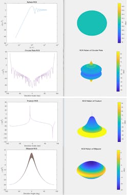
Simple shapes can be used as a proxy for object characteristics. Figure 2 shows other common shapes that are usable as target building blocks. These include a sphere, cone, circular plate, and an ellipsoid. Such shapes can be combined to form more complex scatterers.
2. These are RCS patterns of basic shapes.
RCS of Extended Targets with Multiple Scatterers
Let’s look at a simple multiscatterer case in more detail. The scatterers in Figure 3 are located at the four vertices of a square. Each scatterer is a cylindrical point target as shown earlier. Figure 3 also shows how the RCS of the point target varies when it’s represented by multiple scatterers.
3. Four scatterers (left) and the resulting RCS scattering (right).
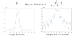
The return received by a radar will vary significantly depending on how many scatterers are present. In Figure 4, you see the results of matched filter processing with a single cylinder versus multiple cylinder scatterers. In this view, the scatterers return multiple signals back to the radar. The signals are brought out through the matched filter of a linear FM chirp waveform.
4. Matched filter of returns with single scatterer (left) and multiple scatterers (right).
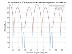
For wideband radars, frequency can also impact the results of what is received by the radar. Wideband radar systems are typically defined as having a bandwidth greater than 5% of their center frequency. In addition to improved range resolution, wideband systems also offer improved target detection. One way in which wideband systems improve detection performance is by filling in fades in a target's RCS pattern. Using the extended target built from four cylindrical scatterers, the modeled narrowband and wideband RCS swept values are shown in Figure 5 as a function of aspect angle.
5. The plots compare narrowband versus wideband returns for a four-scatterer target.
Returns from the multiple cylinders in the extended target model coherently combine, creating deep fades between 40 and 50 degrees. These fades can cause the target to be undetected by the radar sensor.
RCS of Fluctuating Targets
Because the radar system and the target may be moving, the RCS value can change over time. This causes targets to fluctuate. To simulate fluctuating targets, four statistical models, referred to as Swerling 1 through Swerling 4, are widely adopted in practice. The Swerling models divide fluctuating targets into two probability distributions and two time-varying behaviors (see table).
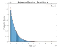
The RCS of a slow-fluctuating target remains constant during a dwell but varies from scan to scan. In contrast, the RCS for a fast fluctuating target changes with each pulse within a dwell. These models apply when the target contains a dominant scattering component. In the Swerling 1 case, the reflection is no longer constant. The RCS value varies from scan to scan. Figure 6 shows the histogram of 10,000 scans with unit incident returns relative to the theoretical calculation.
6. This histogram illustrates a cylindrical target with Swerling 1 fluctuation for 10000 radar scans.
A similar approach can be used to model the RCS of an aerial vehicle, such as a quadcopter. The quadcopter is represented by five scatterers, one for the body of the quadcopter and four for the rotors (Fig. 7).
7. The RCS of an aerial vehicle, such as a quadcopter, can be modeled.
Automotive Radar Example
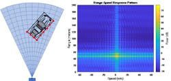
Using a vehicle as an example, you can put together multiple scatterers to form a more complex structure. In Figure 8, you can see the concept in the graphic on the left. The range-Doppler plot on the right shows what the moving vehicle looks like to the radar in the absence of other clutter and objects. These can also be added to the scene to increase the fidelity.
8. Here’s an extended object view of a vehicle (left) and the corresponding range-Doppler view (right).
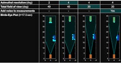
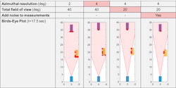
The plot in Figure 8 is based on an IQ-signal-level simulation. Figure 9 shows how detections can also be generated statistically based on a range of factors and radar attributes. These detections are generated from a radar equation-based model. Note how the number of detections (as represented with red circles) changes with different azimuth resolution values, the radar field of view, and the presence of noise.
9. Statistical target detections for an automotive system are based on a variety of factors and radar attributes.
To learn more about the topics covered in this blog, see the links below or email me at: [email protected]
- Modeling Target Radar Cross Section (example): Learn how to model radar targets with increasing levels of fidelity.
- Swerling Target Models (example): Learn how to explore important properties of a signal such as its waveform, spectrum, and ambiguity function.
- Statistical Models for Radars (example): Learn how to model radars with statistical models.
- Model Radar Sensor Detections for Automotive Applications (example): Learn how to model and simulate the output of an automotive radar sensor for different driving scenarios.
See additional 5G, radar, and EW resources, including those referenced in previous blog posts.
About the Author
Rick Gentile
Product Manager, Phased Array System Toolbox and Signal Processing Toolbox
Rick Gentile is the product manager for Phased Array System Toolbox and Signal Processing Toolbox at MathWorks. Prior to joining MathWorks, Rick was a radar systems engineer at MITRE and MIT Lincoln Laboratory, where he worked on the development of several large radar systems. Rick also was a DSP applications engineer at Analog Devices, where he led embedded processor and system level architecture definitions for high performance signal processing systems used in a wide range of applications.
He received a BS in electrical and computer engineering from the University of Massachusetts, Amherst, and an MS in electrical and computer engineering from Northeastern University, where his focus areas of study included microwave engineering, communications, and signal processing.
Honglei Chen
Principal Engineer
Honglei Chen is a principal engineer at MathWorks where he leads the development of phased-array system simulation. He received his Bachelor of Science from Beijing Institute of Technology and his MS and PhD, both in electrical engineering, from the University of Massachusetts Dartmouth.
Rob Graessle
Senior Applications Engineer
Rob Graessle is a Senior Applications Engineer at MathWorks focused on wireless communications, radar systems, and software-defined radio. He previously worked for the Air Force Research Laboratory, Sensors Directorate, and holds a BS and MS from Miami University.
