Model Multi-Domain Simulation Frameworks for Complex Radar-System Designs
Download this article in PDF format.
As radar-system designs become more intricate, the ability to properly model a multi-domain simulation framework is more crucial than ever in terms of influencing decision-making and detecting issues early on in a project. Phased-array antennas are now being used in new designs, ushering in an extended set of capabilities that includes electronic beamsteering and spatial signal-processing techniques.
However, these added capabilities increase system-level complexity. This complexity, coupled with growing levels of interference sources and smaller cross-section targets, is making it extremely difficult for engineers to achieve desired radar performance levels.
Thankfully, radar-system models help to limit the challenges associated with the complexities of today’s design workflow. These models can be used to help justify upgrades to mature, fielded systems before any hardware is procured or developed, and can even assess the lifecycle of a system by understanding how it performs as failures occur—ultimately leading to lower design costs and faster time-to-market.
Explaining the Model
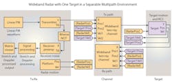
Simulink was used to create a multi-domain, system-level model (Fig. 1). This model covers radar blocks from waveform generation to the transmit/receive chain to the spatial signal-processing components. Environmental and target modeling are also included to complete the system scenario.
1. Shown is a multi-domain radar-system model.
The model shown in Fig. 1 illustrates a low-power X-band radar that can detect targets with small radar cross-section (RCS) values (< 0.5 m2). The required radar coverage for the system in this example is 35 km with a range resolution of 5 meters. This type of radar is typical of a system used to fill gaps within a network of larger surveillance systems.
Each of the building blocks shown in Fig. 1 can also be easily implemented in MATLAB. It’s possible to set up each building block to match the desired system configuration. For example, the waveform description, required transmit power, and antenna gain are parameterized and can be directly configured in each of the blocks. Figure 2 shows sample MATLAB code for radar pulse-level processing.
2. This code was written for radar pulse processing.
Waveform Design
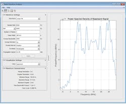
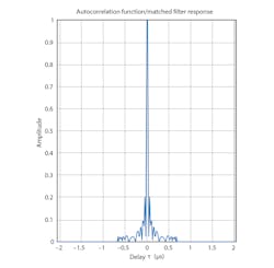
Once the requirements are set for the range and Doppler resolution, as well as the minimum and maximum range of the desired coverage, one can interactively design the appropriate baseband waveform parameters needed to achieve these system requirements. Figure 3 shows a combination of waveform parameters that will achieve the requirements described. The resulting waveform characteristics from these baseband parameters are denoted in the figure to show that the requirements have been met. Figure 4 shows the corresponding matched filter response, which aligns with the performance goals for this system.
3. Users can enter a number of waveform settings.
4. Here is the matched filter response of the radar-system design.
For this type of radar system, the objective is to design a system that requires a low transmit peak power with the intent to translate directly into a lower-cost solution. With lower cost and less system complexity, it should be easier to deploy more systems. The low-power requirement must also be balanced with the need to detect low cross-section targets. Thus, it is required to design an array for the X-band system with a large gain.
Building an Array
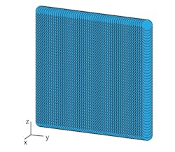
The array parameters, including the geometry, element spacing, lattice structure, and element tapering, can be interactively designed and analyzed. The intended array for the X-band system is a 36-×-36 element array with uniform spacing between each element. Figure 5 shows the resulting array geometry. The radar beam that can be generated with this type of array is able to be steered in azimuth and elevation. An antenna array of this size for X-band is small enough to be easily mounted on a variety of support structures, making deployment of this type of system much easier.
5. This figure illustrates a 36-×-36 uniform rectangular array (URA).
The array design can be directly used in the system model. Due to the large number of elements in the array, the resulting antenna directivity allows the peak power to be less than 20 W. This performance is based on an array directivity of 34.73 dBi. Taylor weighting has been applied to reduce the side-lobe levels.
If a higher level of fidelity in the model is needed, a specific antenna element can be designed using a full-wave solver in Antenna Toolbox. One can also model the effects of mutual coupling between antenna elements, which typically impacts the beam pattern as it is steered off boresight in both azimuth and elevation. As a result, one can easily see how the array design affects the performance, making it possible at an earlier stage to either change the design or adjust the requirements for downstream processing.
"What If" Analysis
Before moving on to some of the other radar blocks, it is interesting to note that the model can also be used to support a variety of specific "what-if" analysis exercises that relate to more detailed design tradeoffs and lifecycle planning. For example, the framework in place can be referenced for the best implementation of array-thinning techniques.
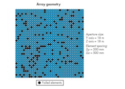
6. Shown is a 36-×-36 array with failed elements.
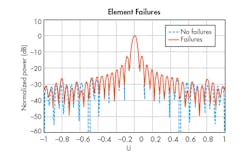
Alternately, Figures 6 and 7 show one way to evaluate the impact of failed elements in the array. This evaluation can be important for determining maintenance cycles. For a radar site that is not staffed 24/7, multiple failures can be tolerated before a site is visited and the failures are repaired. Fig. 7 shows the degradations in the beam pattern with 15% of the elements failed.
7. These plots show how element failures affect the beam pattern.
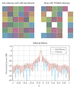
Similar analysis can be performed at the subarray level as well. Figure 8 illustrates the array built up from 6-×-6 subarrays. The resulting beam pattern is also shown, with 10 of the 36 subarrays in a failed state. Again, this type of data can be used to determine how many subarrays should be implemented. Moreover, it can be utilized in a way similar to the maintenance concept described earlier.
8. This figure illustrates a 36-×-36 element array that is built with 6-×-6 subarrays. The beam pattern is shown with no failures, as well as with 10 failed subarrays.
Modeling a Complete Scenario
Tools are available for each component to help quickly complete a system model. In this example, targets of varying complexity (including RCS fluctuations and angle- and frequency-dependent RCS behavior) are created. These targets can also be set in motion in the model. This capability provides insights into whether the design meets all performance goals. Various factors, such as line-of-sight propagation effects due to rain, fog, and gas, as well as channel fading, can be included to improve the model’s fidelity.
To emulate the complex RF environment, it’s possible to integrate signal-source models to test interference mitigation techniques and assess complexity levels prior to implementation. In this model, targets are added with an RCS value of 0.05 m2. This type of scenario has taken on new importance with the increased use of drones and unmanned aerial vehicles (UAVs).
In addition, fidelity in the RF domain can be extended by building up subarrays with models of RF components, such as phase shifters, amplifiers, etc. Simulink can serve as a platform to perform multi-domain simulation because it provides customizable block libraries and solvers for modeling and simulating dynamic systems. Since it is integrated with MATLAB, one can incorporate algorithms into models and export simulation results to MATLAB for further analysis.
Forming Multiple Beams
In this signal-processing subsystem, multiple beams are formed that cover various azimuth and elevation angles in front of the array. These same channels also estimate the directions that the returned signals are arriving from. The matched filter shown in Fig. 4 provides the system with a processing gain that improves the detection threshold. A time-varying gain is added to the model so that a constant threshold can be used for detection across the entire detectable range.
The resulting pulses are non-coherently integrated. The combination of these techniques allows processed returns for a single integration interval to support target detections at a desired signal-to-noise ratio (SNR). Results can be visualized in a variety of ways, including power vs. time and intensity vs. time.
In this example, the simulated targets have a non-fluctuating RCS of 0.5 m2 and are located throughout the area of radar coverage. It should be noted that the blocks used in the simulation are scalable. Each input and output is clearly defined such that custom blocks can be swapped into the model or extended to an existing block. Among the resulting data sets from the model is I/Q data generation for each processing interval.
Assessing Radar Network Coverage
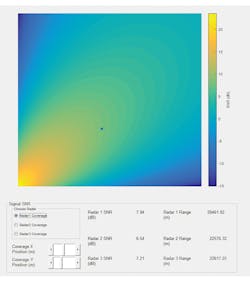
9. This is the SNR view for one of three radar systems.
By using this model as a starting point, one can also investigate ways to perform analysis on potential networks of radars. For example, consider a simple configuration of three systems that are placed with overlapping coverage to avoid any gaps. Figure 9 illustrates the SNR in one of the three coverage areas. A SNR of at least 5 dB is the goal given the combination of signal processing and integration that was implemented.
Time and Cost Savings
While off-the-shelf radar model components provide all of the basic building blocks for a full system model, the simulation framework also has the flexibility to be extended with custom additions for each portion of the radar design. As demonstrated in the examples, the radar-system design workflow, from requirements analysis to design tradeoffs to system development, can benefit from this work.
Modeling such an elaborate radar system early in the design process is able to save countless hours and reduce program costs by exposing design issues in the early stages of the project. Furthermore, a full system model can simulate a radar system for signal-processing development or generate the radar echo(s), resulting in I/Q data that can be tuned to algorithms. After tuning the algorithm, it is easy to replace the synthesized data with measured data at any location in the model, speeding up development processes and saving cost on future designs as well.

